We are using this: Light_Atom-2011.11.24.pdf
- download it!
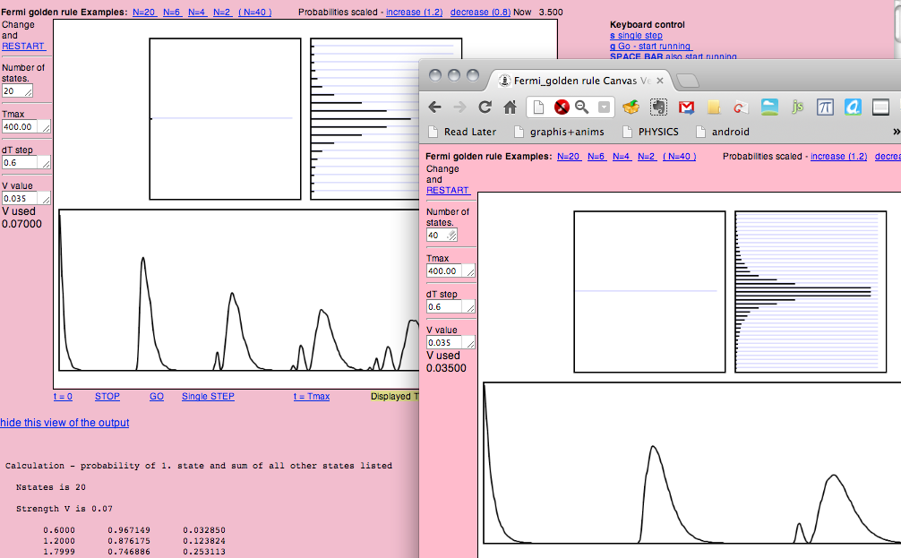
We worked with http://web.ift.uib.no/AMOS/golden/
Try it!
Picture-page about Fermi Golden Rule
http://web.ift.uib.no/~ladi/Fysisk/Teori/Pictures/Golden.html
Quantum mechanics -
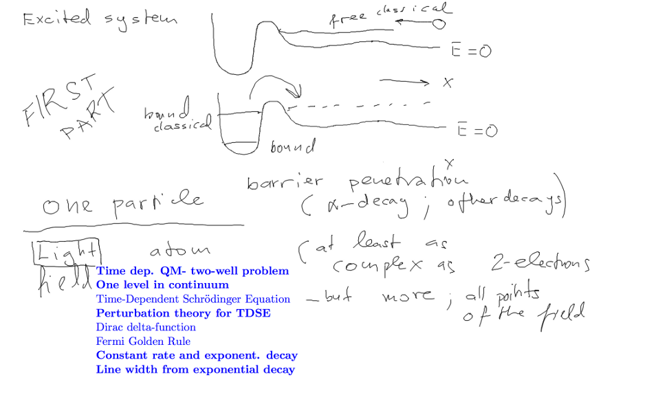
non-stationary, time dependent: Main type of phenomena - DECAYS
alpha-decay as example.
Two "regions" - Probability streaming from one region to the other;
exponential decays, see below
0-time-in-QM-decaying-states-alpha-decay-etc.png
0-time-in-QM-decaying-states-alpha-decay-etc.png
The parts of our note which cover this part (blue text, from the
"Topics" page of Light_Atom-2011.11.24.pdf
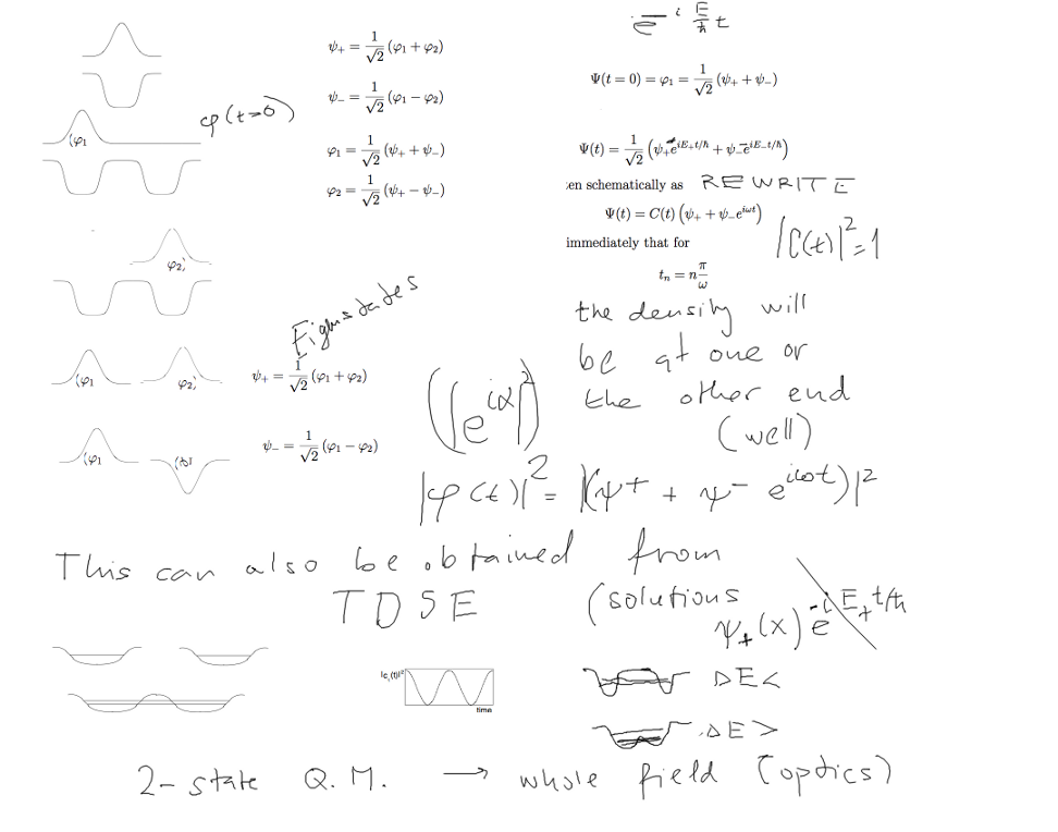
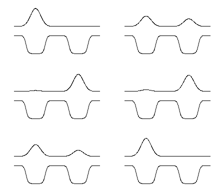
Two regions - model - two-states
One particle can be in two (equivalent) regions - probability will
oscillate
1-time-developement-two-well-2-state.png
1-time-developement-two-well-2-state.png
 animAAA.gif
One region has many states, the first one has still one state -
initially prob. one - then decay
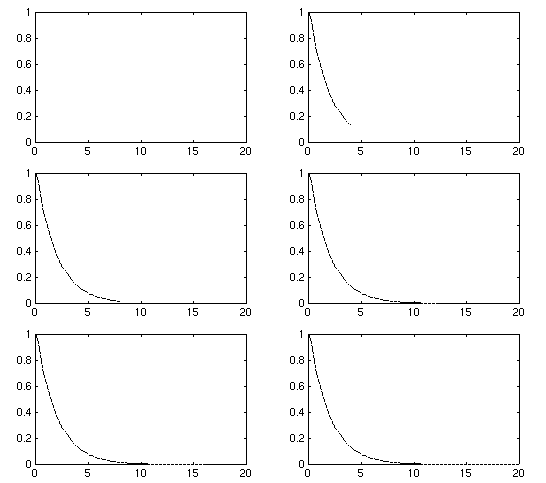 animRUL.gif
  3-two-wells-Decay.png
In the following we shall discuss what we usally find in
textbooks: Time dependent perturbation theory
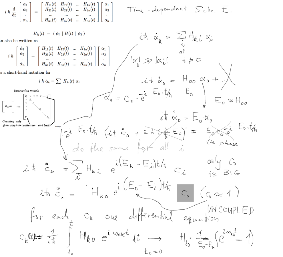
Transform Time dependent Schr. EQUATION to coupled differential
equations for amplitudes/expansion coefficients
Perturbation -> assumptions about small changes
2-Time-dependent-Schroedinger_EQ---TDSE.png

2-Time-dependent-Schroedinger_EQ---TDSE.png
With those assumptions equations decouple and the solutions are
straightforward inegrations
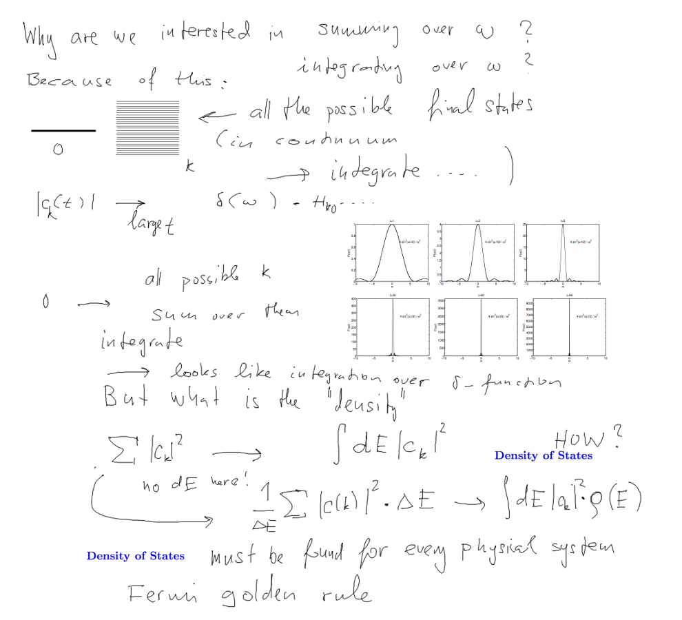
Summing over the final states - see our simulator illustrations
(continuum, represented as limit of equally spaced )
3_Fermi_Golden_Rule.png

3_Fermi_Golden_Rule.png
How does it become "like a delta-function" -
AND THE ORIGIN OF DENSITY OF STATES factor
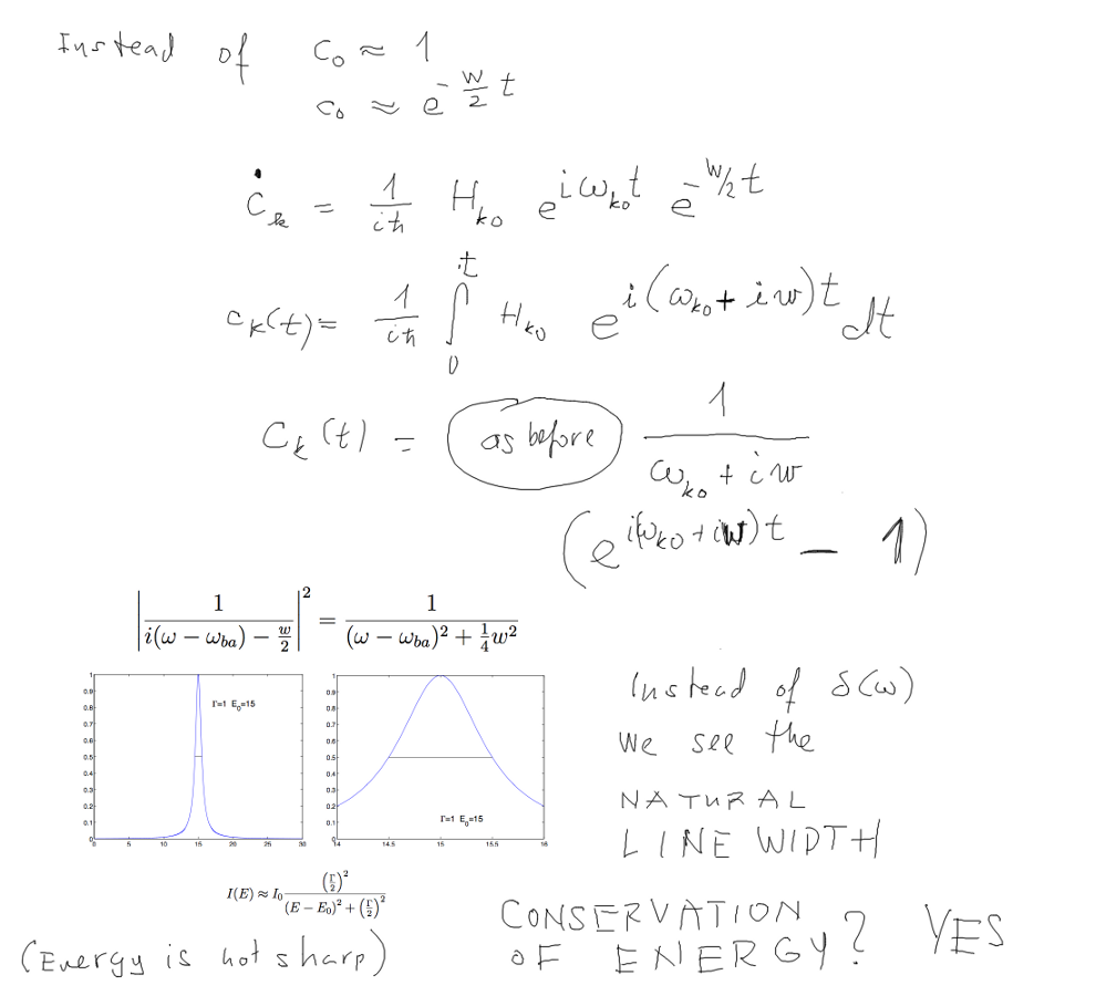
BUT LINES ARE NOT SHARP, NO DELTA FUNCTIONS
4_Modify_Dirac_delta_to_Lorentz_line_profile.png

4_Modify_Dirac_delta_to_Lorentz_line_profile.png
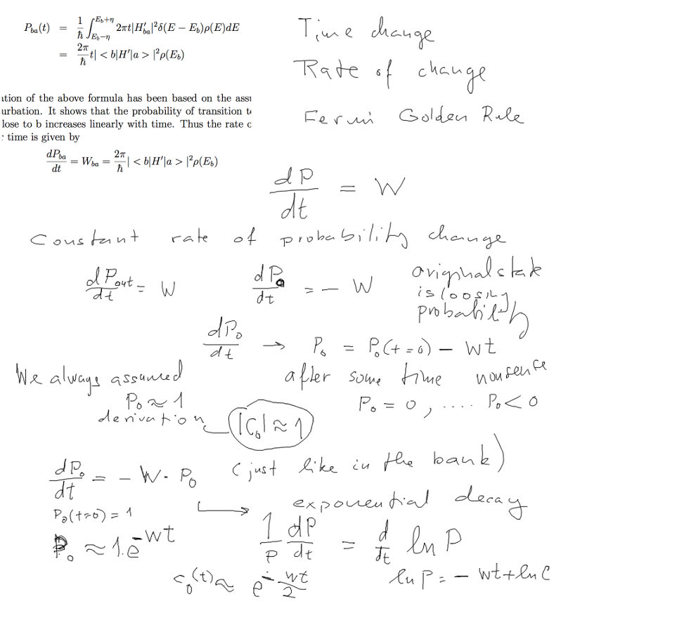
HERE WE SHOW HOW THE constant rate of change leads to a more
realistic model
of exponential decay - the relation must be modified
5_Modify_Dirac_delta_to_Lorentz_line_profile.png

5_Modify_Dirac_delta_to_Lorentz_line_profile.png
The Lorentz line - shape is general, present in all fields of
physics.
The formula is also known as Breit-Wigner formula - for
RESONANCES ( nearly all elementary particles appear as RESONANCES )
ALSO similar to the driven classical oscillator
To understand the time-development, we have several versions of
"Fermi Golden Rule simulator"
One is in a web-page, shown below, others are in Matlab
http://web.ift.uib.no/AMOS/golden/
EXERCISE: play
with the web-simulator, some hints will be provided later
with recurrencies
(a special case;) ( recurrences come because our spectrum is
not truly continuous ;
recurrencies happen in fact in some physical systems and have been
observed - i.e. particle re-appears ..... new research )
z-capture-Fermi_Golden.png

z-capture-Fermi_Golden.png
Quantum Mechanics of time developement - part 1 We are using this: Light_Atom-2011.11.24.pdf
- download it!
We worked with http://web.ift.uib.no/AMOS/golden/
Try it!


 animAAA.gif
 animRUL.gif
  3-two-wells-Decay.png