Interaction of Atoms with Light - Part 3
The PDF-file of the presentation : Light_Atom-2013.10.16.pdf
SCF-exercise COMMENT at the end
1.
Time-dependence in quantum mechanics - probability rate - short comment
2. Eigenmodes /
Normal modes
3. Operator method for harmonic
oscillations - creation/annihilation operators
We started with a small review of
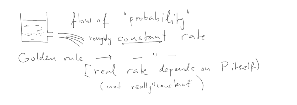
the time-dependence - Golden Rule - And why the "constant rate" case
depends on "how much is
left" - Illustration by analogy of a flow out of a jar
010_constant_rate_depends_on_content.png

010_constant_rate_depends_on_content.png
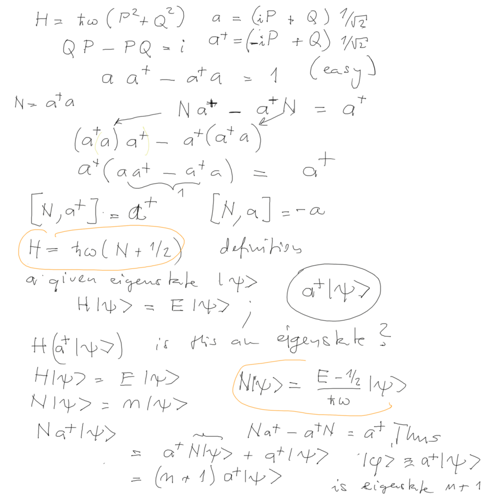
Operator method for harmonic
oscillations - transforming to dimensionless Q, P -
energy h omega outside
Q,P can be combined to a and a+ -
commutation relations - and suddenly we can construct the "NUMBER
OPERATOR"
H is proportional to N, thus we only need to work with the
combination a , a+ and N= a+ a
Provided we know an eigenstate - apply a+ or a
to it - and it turns you get a NEW eigenstate of N with value n+1
or n-1
020_operator_method_for_Harmonic_oscillator.png

020_operator_method_for_Harmonic_oscillator.png
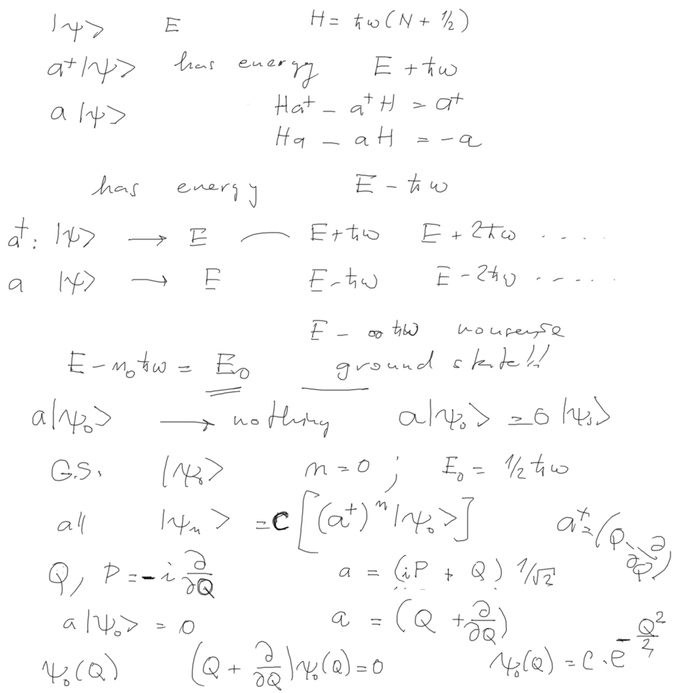
Operator method for harmonic
oscillations - continue
Thus a and a+ are LADDER¤ operators
AT the end we obtain a MUCH simpler differential equation for the
ground state
Algebraic method for Harmonic oscillator is elegant, but also very
important
--- it provides the creation - anihilation operator
formalism
030_operator_method_for_Harmonic_oscillator.png

030_operator_method_for_Harmonic_oscillator.png
Operator method for harmonic
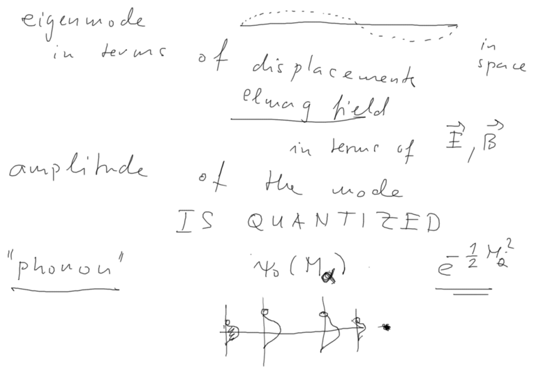
oscillations - normal modes - QUANTA
creation operator "creates a quantum" of energy of the "mode"
PHONON - or perhaps also PHOTON ?
Towards the end we started to discuss the spatial distribution of a
normal mode "wavefunction"
in real space coordinates, not in the normal coordinates
040_creation-annihilation_phonon_and_photon.png

040_creation-annihilation_phonon_and_photon.png
Here are normal coordinates
demonstrated in MATLAB. Matlab finds the eigenvalues and eigenvectors
for a coupled string. IT TURNS OUT
THESE ARE KNOWN ANALYTICALLY (Toeplitz Matrix, see later)
- but Matlab just does it quickly.
There are "quasicontinuously" distributed eigenfrequency values
OMEGA Squared
- and corresponding eigenvectors - the eigenvectors are plotted.
They show the eigenmodes as distributed
over "the string" - it really resembels the eigenmodes of a
string (gitar or piano string ...)
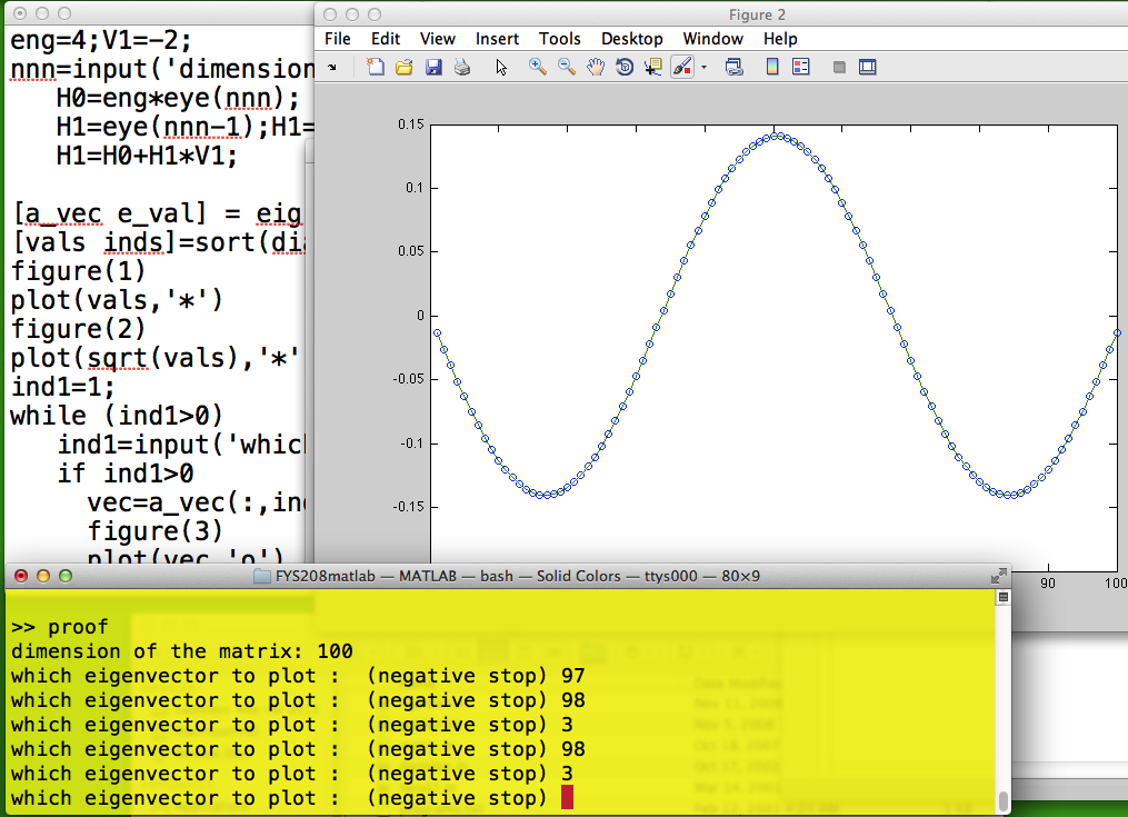
N=100 in both cases below, i.e. string of 100 balls
205_n_3_Oscillator.png

205_n_3_Oscillator.png
Above and under: above - the third lowest frequency
n=3
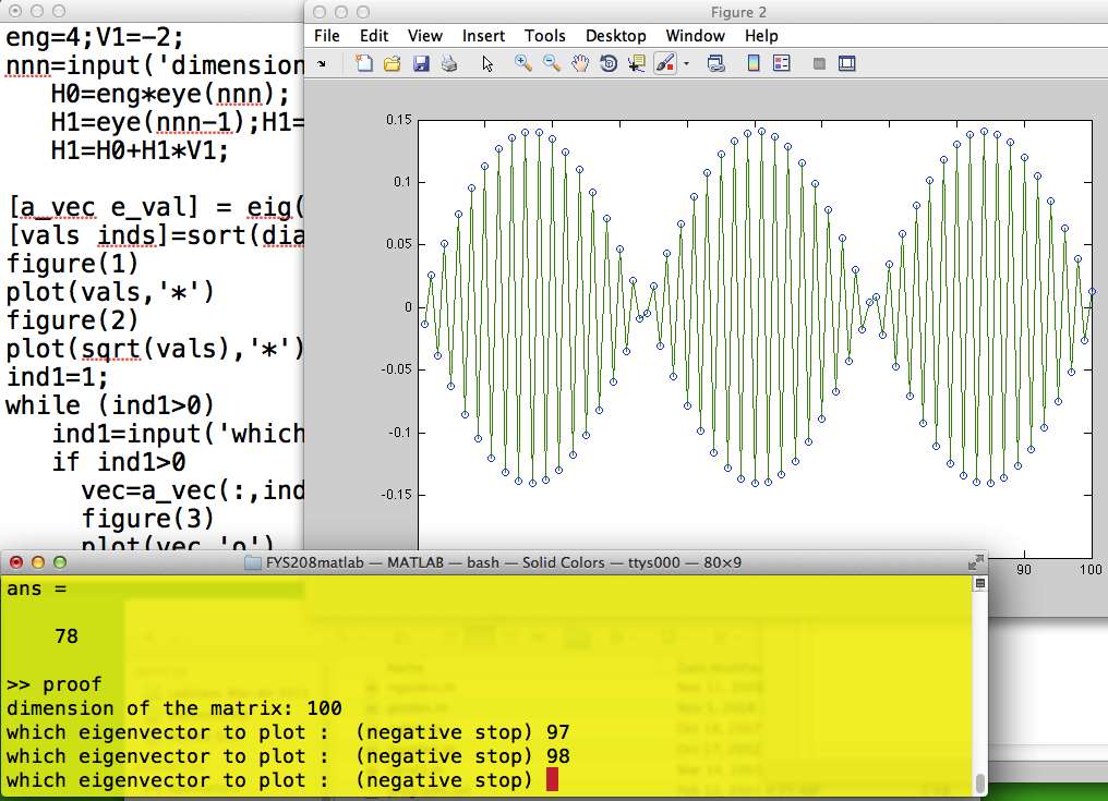
under the third highest frequency - the lines are drawn to show the
neighboring displacements n=98
N=100 in both cases below, i.e. string of 100 balls
210_n_98_Oscillator.png

210_n_98_Oscillator.png
Discussion of how the vibration's - photon's wavefunction looks
like in the normal space,
i.e. in terms of the INDIVIDUAL DISPLACEMENTS (classically - simply
what shown above, MATLAB)
Quantum case - more complicated? Wavefunctions?
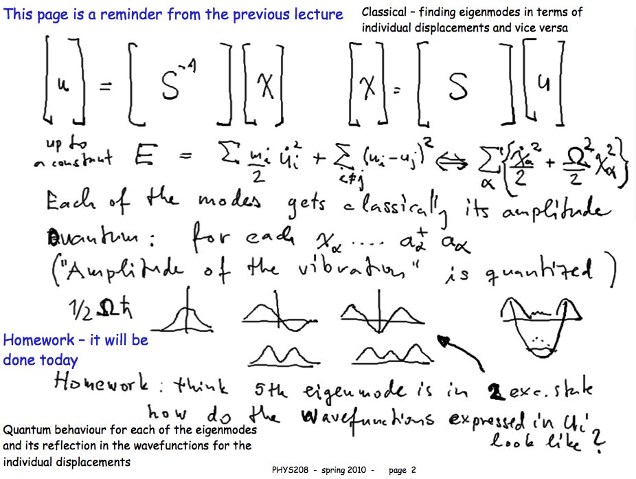
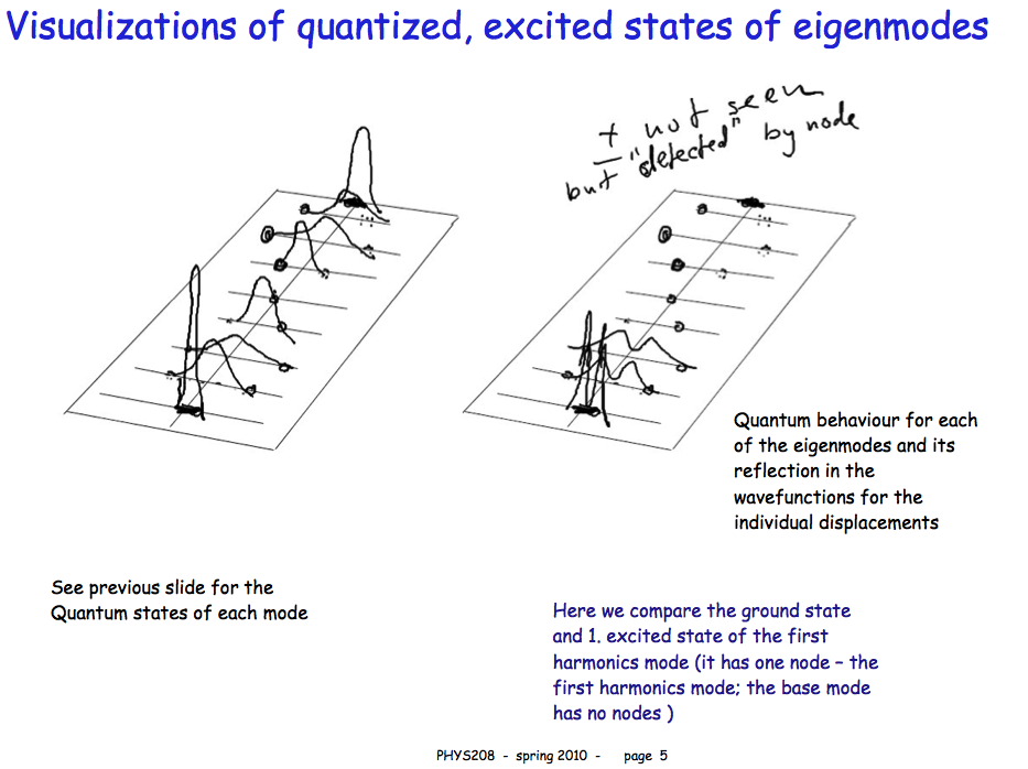
These board-shots are from a solid state lecture - spring 2010
110-normal-modes-eigenmodes.png

110-normal-modes-eigenmodes.png
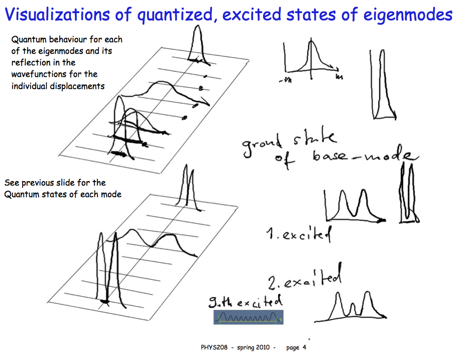
These board-shots are from a solid state lecture - spring 2010
It turns out that these drawings are in fact not quite correct - useful
for discussion anyway
120-Harm.Osc.States-and-normal-modes.png

120-Harm.Osc.States-and-normal-modes.png
These board-shots are from a solid state lecture - spring 2010
It turns out that these drawings are in fact not quite correct - useful
for discussion anyway
see a correct description below
130-Harm.Osc.States-and-normal-modes.png

130-Harm.Osc.States-and-normal-modes.png
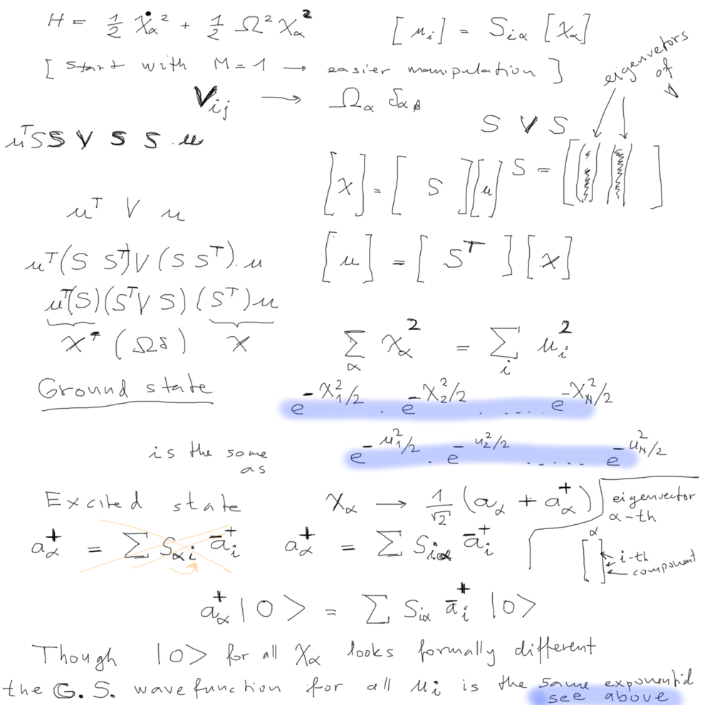
Here is the lecturer's HOMEWORK (not yet at the lecture)
first slide - the formal operations clarified, The eigenvectors
arranget in matrix S,
the transposed matrix is also an INVERSE matrix - from the definition
of normalized
eigenvectors
140_Harm_osc_2013_explanation.png

140_Harm_osc_2013_explanation.png
Ground state of all the normal modes - and then written in terms of the
individual displacements
(blue-outlined parts)
What are the "individual" a+i -
creations of vibrations with the MODE FREQUENCY but displacement in the
given point
THEY ARE NOT real vibrations of the given ball - those would have all
the independent vibration frequency.
They "do not exist" - system is strongly coupled, no uncoupled are
reasonable
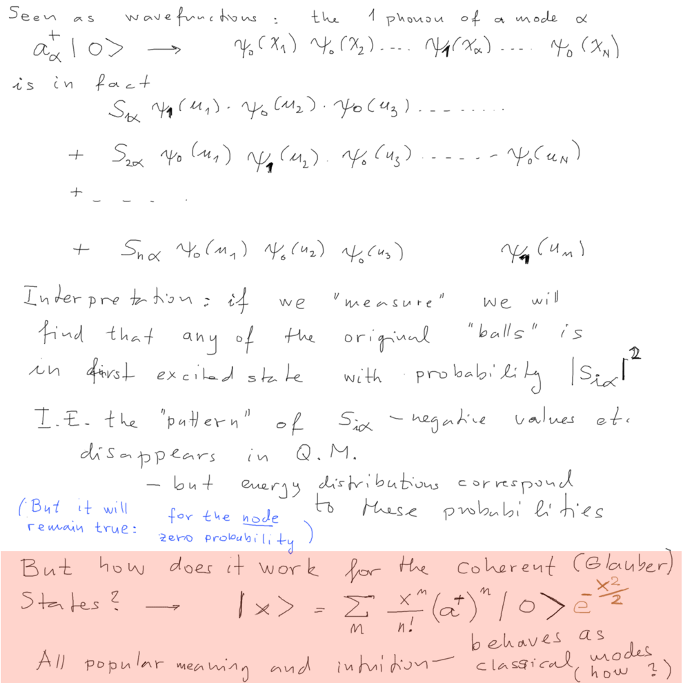
Here is the correct explanation of how the 1 (static) phonon state
looks like
alpha-th eigenmode, all other modes in their ground state
Then use the transformation compare with definition above - and read
the explanation below
150_Harm_osc_2013_explanation.png

150_Harm_osc_2013_explanation.png
The "photon" is smeared out - it is a sum of many terms, in each term
the oscillation is concentrated in one "ball" displacement
- with amplitude following from the eigenmode.
In terms of probabilities: we would measure distribution of values of
the displacement of the i-th ball
to be just like the width of the 1. excited state with probability
amplitude squared - as shown - call it P(i).
It will be found to correspond to its "ground state" with
the probabilty of squared sums remaining - which is 1- i.e.
1-P(i)
---- a bit
difficult to plot
----- see also above --------
What are the "individual" a+i -
creations of vibrations with the MODE FREQUENCY but displacement in the
given point
THEY ARE NOT real vibrations of the given ball - those would have all
the independent vibration frequency.
They "do not exist" - system is strongly coupled, no uncoupled are
reasonable.
The last/colored part: about coherent states; see lasers later on
COMPUTATIONAL EXERCISE
DISCUSSION
A more detailed project is described here
../2011_09_27/SCF-Herman-Skillman/index.html
in particular the fitting (guessing) of the Z-dependence
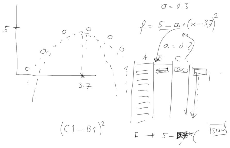
There are many tools and simple methods to do such "variational"
procedure
We have looked at how to do it in a SPREADSHEET - using a function
definition
This is what remained as a note:
300_how_to_fit_z-dependence_spreadsheet.png

300_how_to_fit_z-dependence_spreadsheet.png
LECTURE NOTE 2013.10.29
to index
2013.10.17 -
previous lecture note
2013.11.05 - next lecture
note
