1. Review the basics of time development
2. Time dependent perturbation theory - to derive Fermi Golden Rule
3. The issues of "energy conservation" - the natural line width ( refer to "the eigenstates" last time )
4. Density of states - from k-space to energy integral
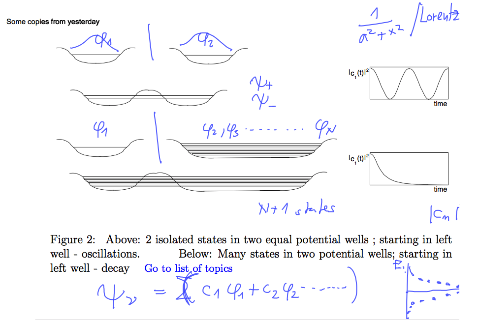
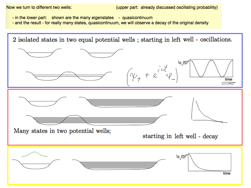
The difference between the 2 "identical wells" and one level "embedded in quasicontinuum"
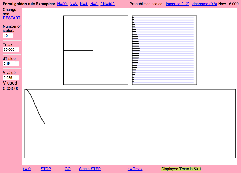
Oscillations vs decay
sc_0100.png
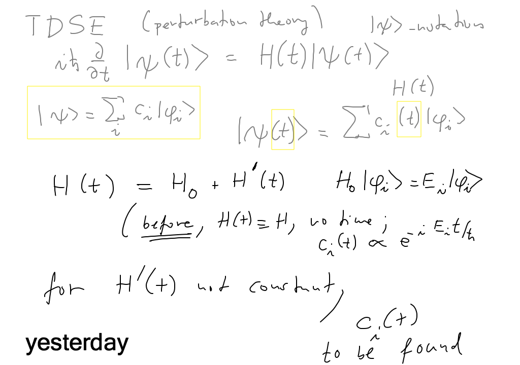
TDSE - Time-dependent Schrödinger Equation
Either perturbation theory - usual in QM courses
or
Expansion in a basis - and perturbation theory
or
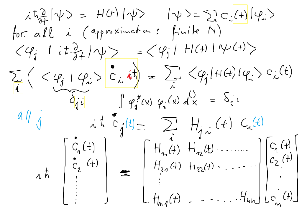
Coupled differential equations for the expansion coefficients - As we do here
sc_0200.png
This method is widey used in many areas of quantum physics
Jump to the perturbation discussion here - slide sc_1300.png
sc_0300.png
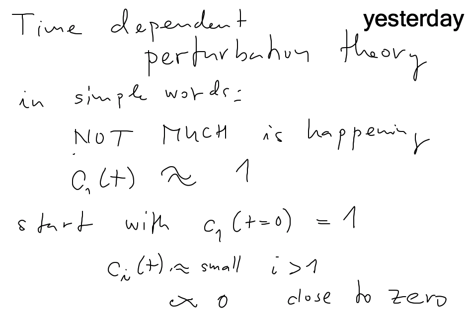
The method also used as syarting point of TIME DEPENDENT PERTURBATION THEORY
Jump to the perturbation discussion here - slide sc_1300.png
sc_0400.png
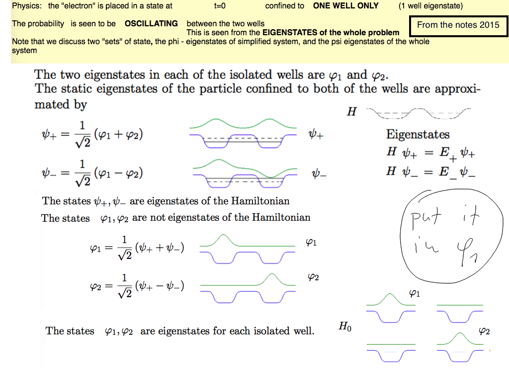
Returning to the two "identical levels" and one level "embedded in quasicontinuum"
in the next plate in a formal way.
sc_0500.png
Once more - as in the last lecture
sc_0700.png
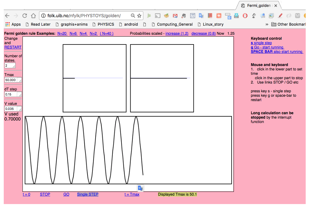
Golden rule simulator http://folk.uib.no/nfylk/PHYSTOYS/golden/
here used to show the N=2 two-well oscillation
 sc_0810.png
Returning to the 2 types of expansion
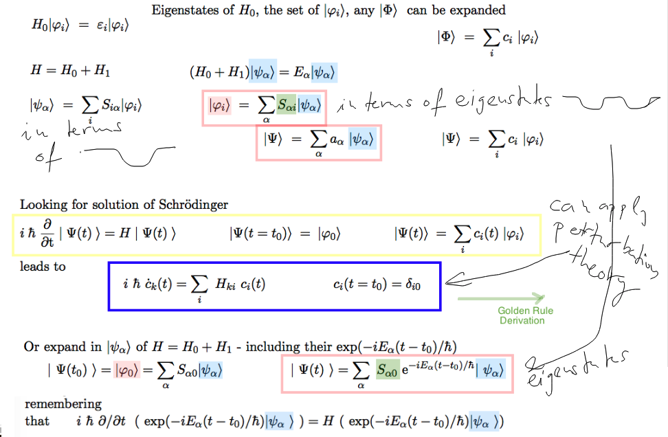
sc_0900.png
Returning to the 2 types of expansion
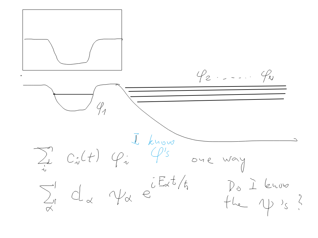
sc_1000.png
Returning to the 2 types of expansion - here explained in detail
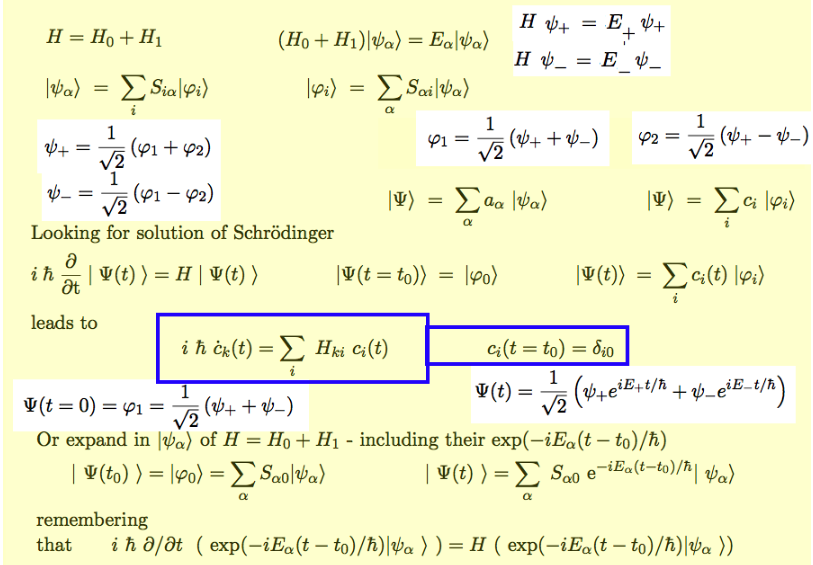
sc_1100.png
The eigenstates - the "component" of the initial single state is distributed as in the "natural line width"
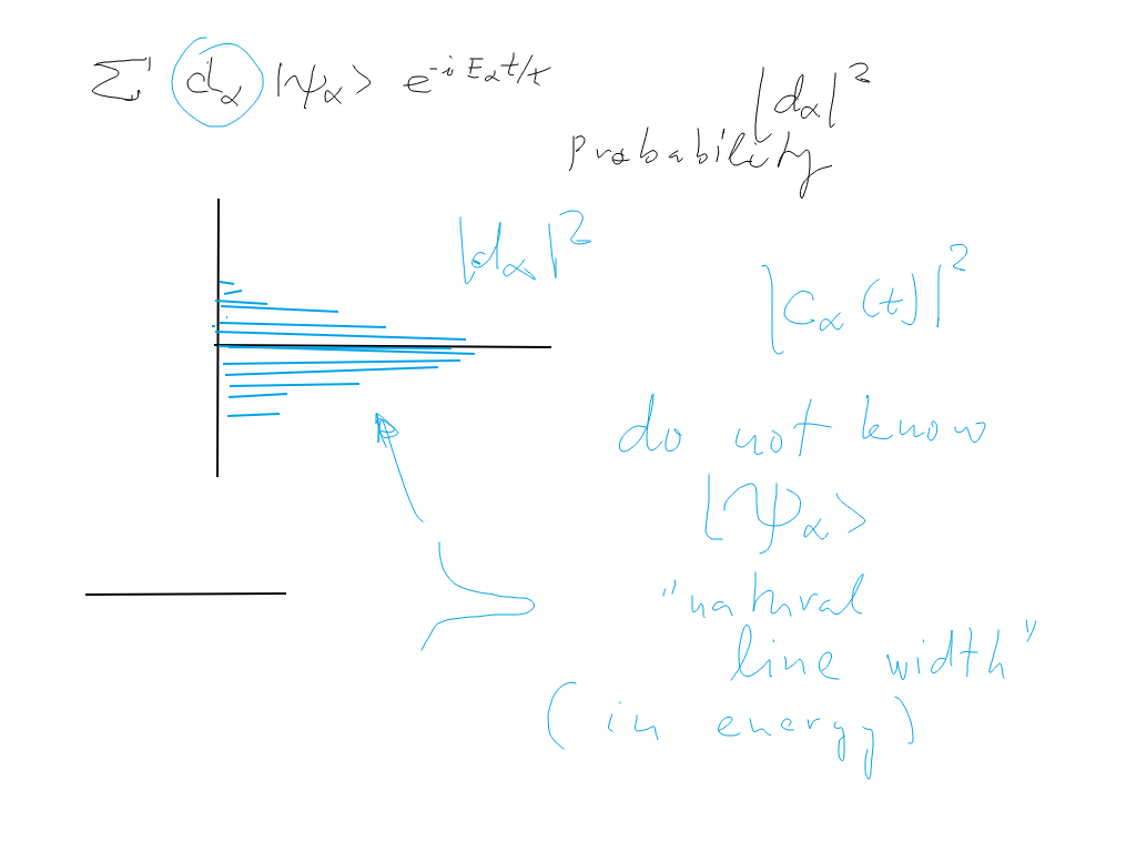
sc_1200.png
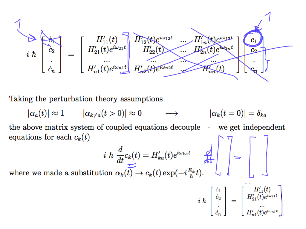
"Time dependent perturbation theory" - without too much "theory".
We just assume that something is much smaller
Then we cut away the small things; keep only the dominant ones
Here we are taking the above slide sc_0300.png and cut away the small parts
The "smallness" assumptions are listed
sc_1300.png
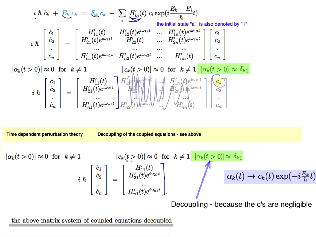
This is the reduction done explicitely
sc_1400.png
No coupled equations; Also, not any first order term, ONLY THE DERIVATIVES are remaining
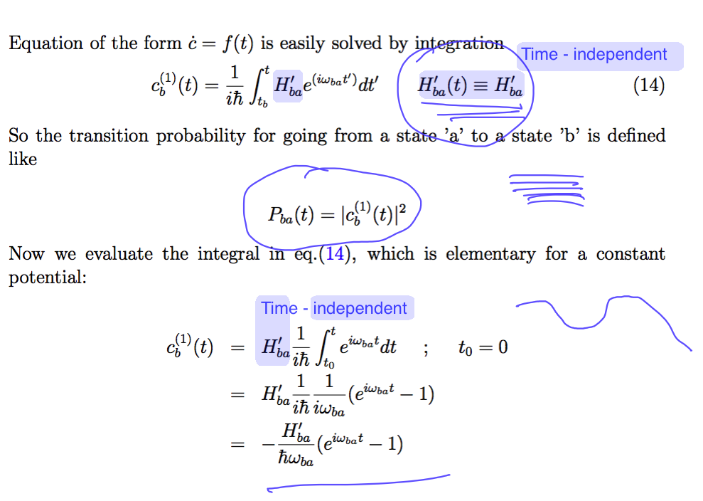
Such Diff. Eq. are very easily solved - just integrate
sc_1600.png
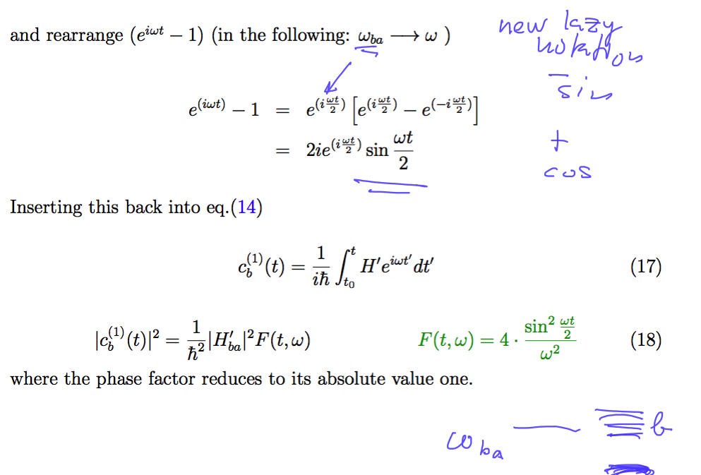
another step - get a phase times sine
Getting the function of t and omega ( i.e. the ENERGY DIFFERENCE omega )
sc_1700.png
The function F works as a Dirac delta-function - if we want to integrate over it
Do we want to integrate over it?
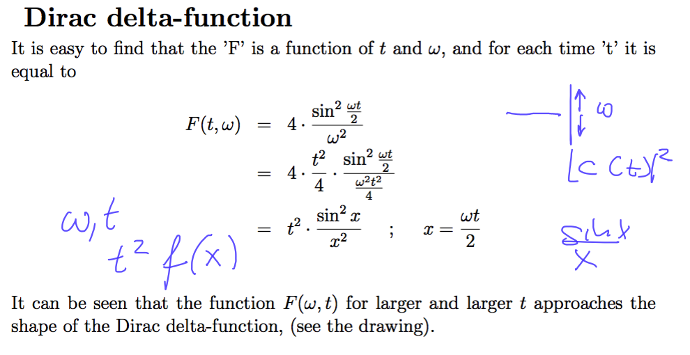
sc_1800.png
The delta function - as the time increases (to infinity ... or eternity .... )
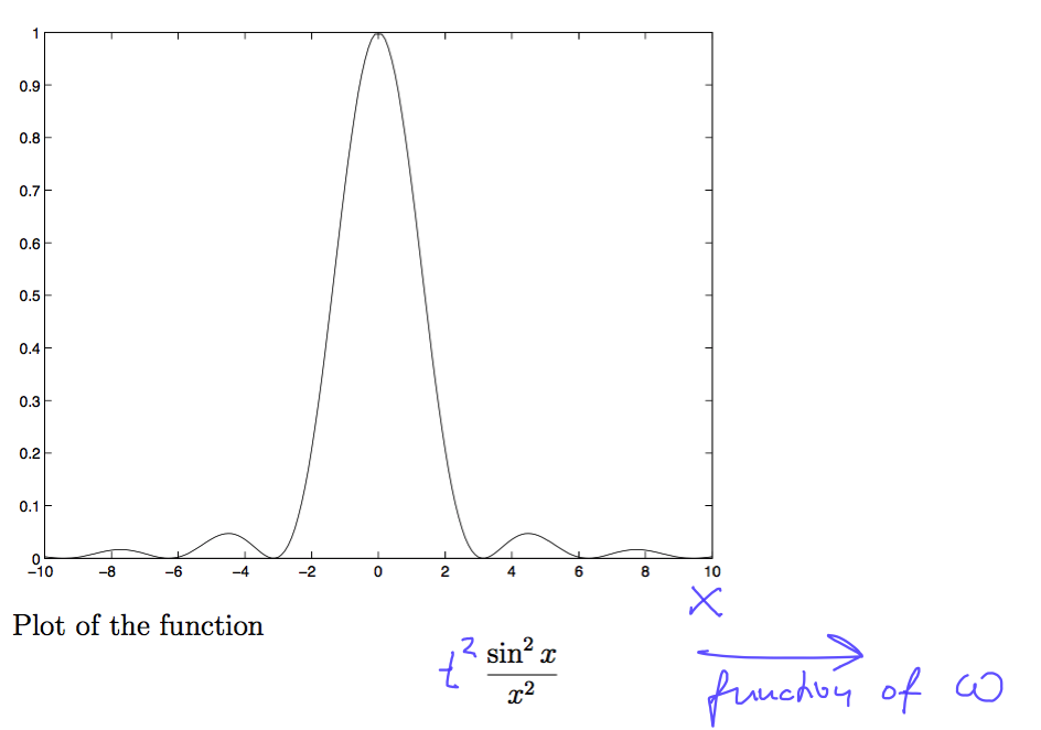
sc_1900.png
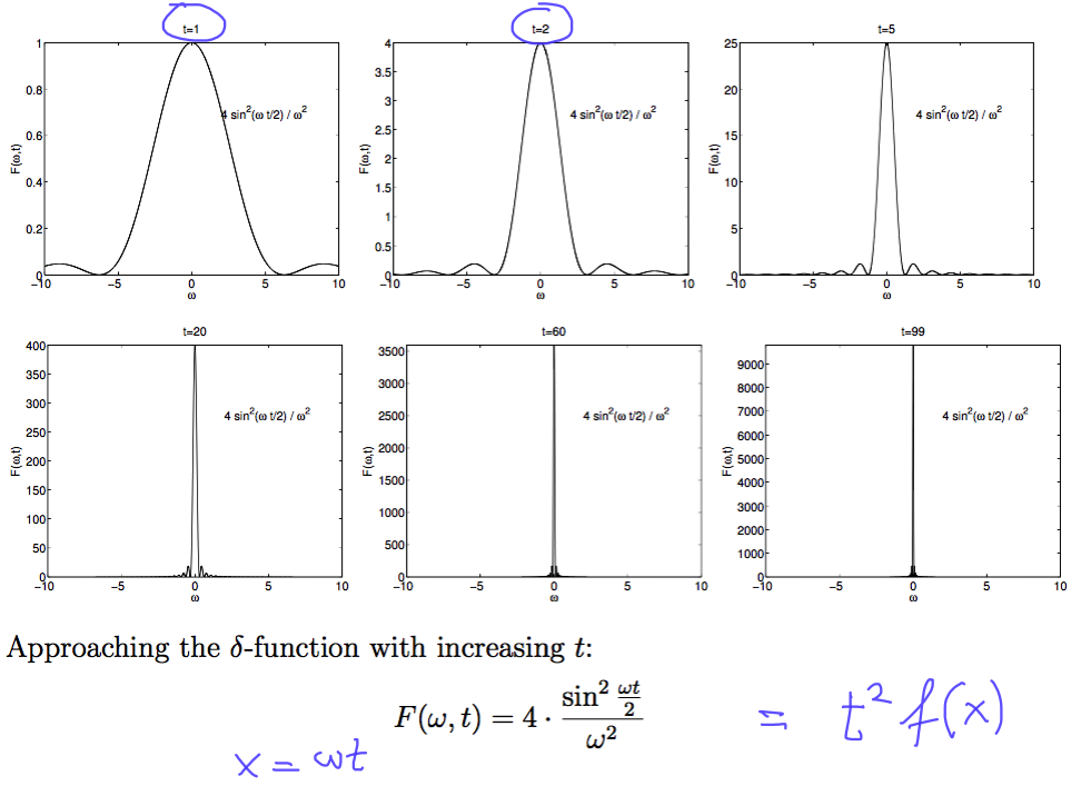
sc_2000.png
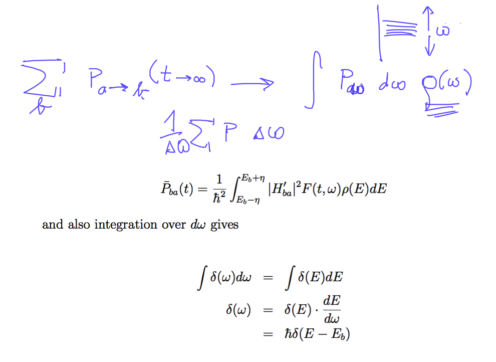
so why we want to integrate ( we want to "sum" over the "quasicontinuum" - where the probability leaks to )
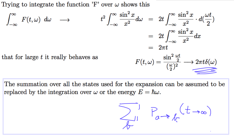
sc_2100.png
Once more with more detail:
so why we want to integrate ( we want to "sum" over the "quasicontinuum" - where the probability leaks to )
sc_2200.png
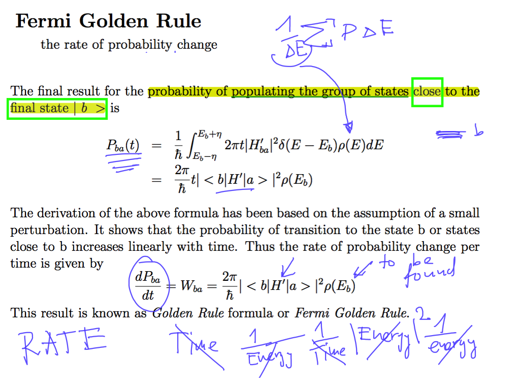
And here we get the Golden Rule
sc_2300.png
Perturbation theory assumption and golden rule - can not be "correct" for all times - it is an approximation
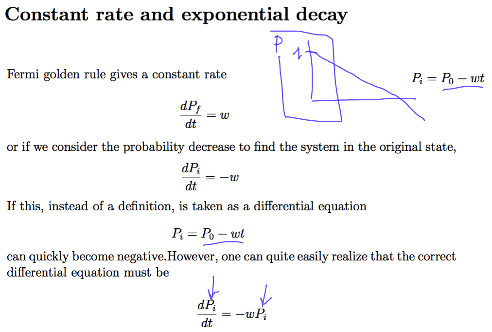
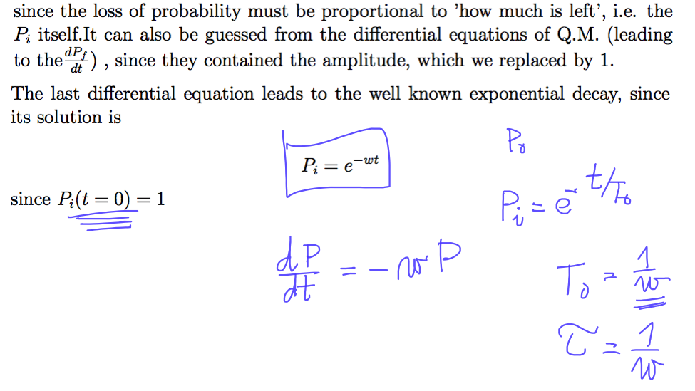
Exponential decay
sc_2400.png
sc_2500.png
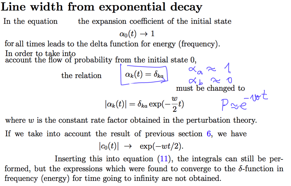
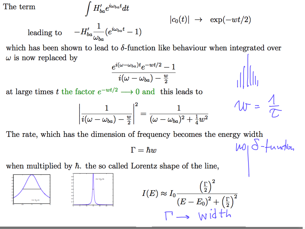
To get the Line width - the assumption about the unchanged close to 1 coefficient must be replaced by exponentially decrease
sc_2600.png
sc_2700.png
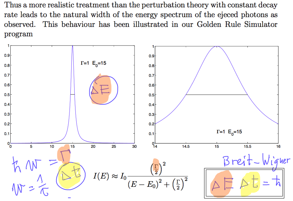
Line width - Lorentz profile ( Breit-Wigner and resonances )
Our discussion of the "quasi-continuum eigenstates" explains the line width
The eigenstates-expansion (stationary states!) - see this comment in the last lecture - link here
sc_2800.png
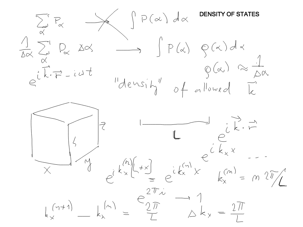
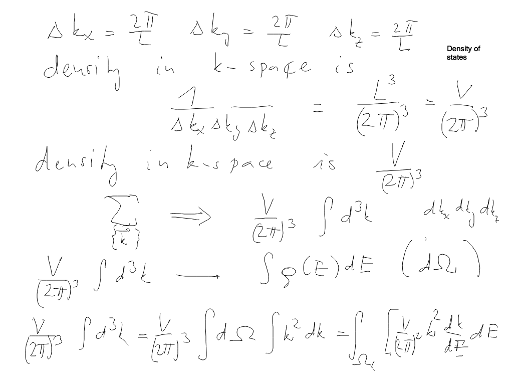
Density of states - from k-space to energy integral
whenever we go to an integral from a sum
we must get the "density of states" factor
sc_2900.png
Integral contains Delta tau ( in limit) but the sum has no Delta tau
Thus the sum is Integral (containing Delta tau) / delta tau and 1 / Delta tau IS the density of states ( why ?! )
sc_3000.png
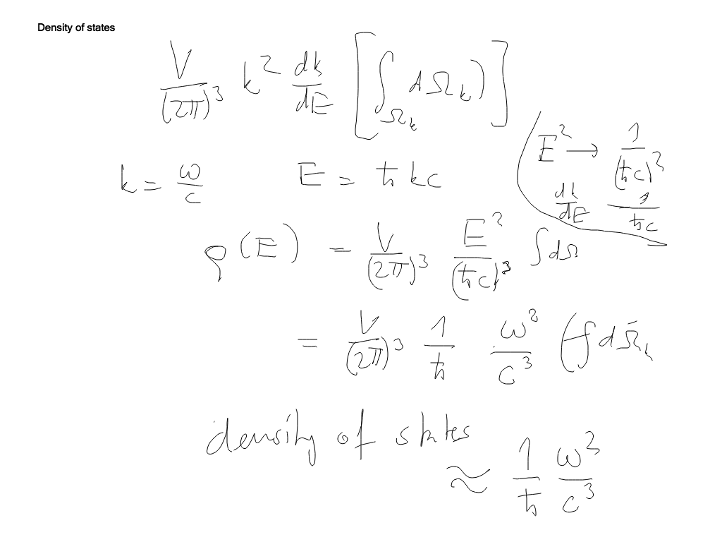
The factor density of states obtained - but the angular (directional) integration is left unperformed
We should actually talk about the density of states "emerging" in an element of solid angle
probability per one Energy unit and per sterradian ....
sc_3100.png
NEXT: extended systems - fields - vibrations - EIGENMODES / NORMAL MODES
Harmonic oscillator and Quanta - "second quantization"